Convection
0 ContainersFiles in Convection
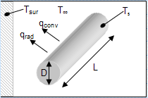
Annual cost of heat loss through pipes.xls
KNOWN: Length, diameter, surface temperature and emissivity of steam line. Temperature and convection coefficient associated with ambient air. ...
Cartridge heater - Heater power - Convection coefficients in air.xls
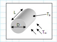
KNOWN: Dimensions of a cartridge heater. Heater power. Convection coefficients in air and water at a prescribed temperature. FIND: Heater ...
Compare convection coefficients for the water and air flow.xls
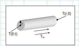
KNOWN: Long, 30mm-diameter cylinder with embedded electrical heater; power required to maintain a specified surface temperature for water and a...

Drag force in air flow.xls
KNOWN: Air flow conditions and drag force associated with a heater of prescribed surface temperature and area
FIND: Required heater po...

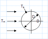
External Flow Over Cylinder.xls
Purpose of calculation: Calculate convective heat transfer for a cylinder in cross flow at various velocities. Input cells in blue. ...
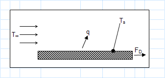
Power required to overcome drag force at a given velocity.xls
KNOWN: Air flow conditions and drag force associated with a heater of prescribed surface temperature and area.
FIND: Required heater p...
Time to heat shaft to a given temperature.xls
KNOWN: Diameter and radial temperature of AISI 1010 carbon steel shaft Convection coefficient and temperature of furnace gases.
FIND: ...