ODE - Initial Value Problem using Euler's Method

Full Description of How This Calculation Works

The Mathematical Foundation

Euler's Method is the most fundamental numerical technique for solving ordinary differential equations (ODEs) when you know:

1. A starting point (initial condition): x₀, y₀
2. How the function changes (the differential equation): y' = f(x, y)
3. Where you want to go (target value of x)

The Step-by-Step Process

Given:

• Differential equation: y' = e^(-4y + 2x)
• Initial condition: At x = 0, y = 0
• Step size: h = 0.05
• Goal: Find y(1.2)

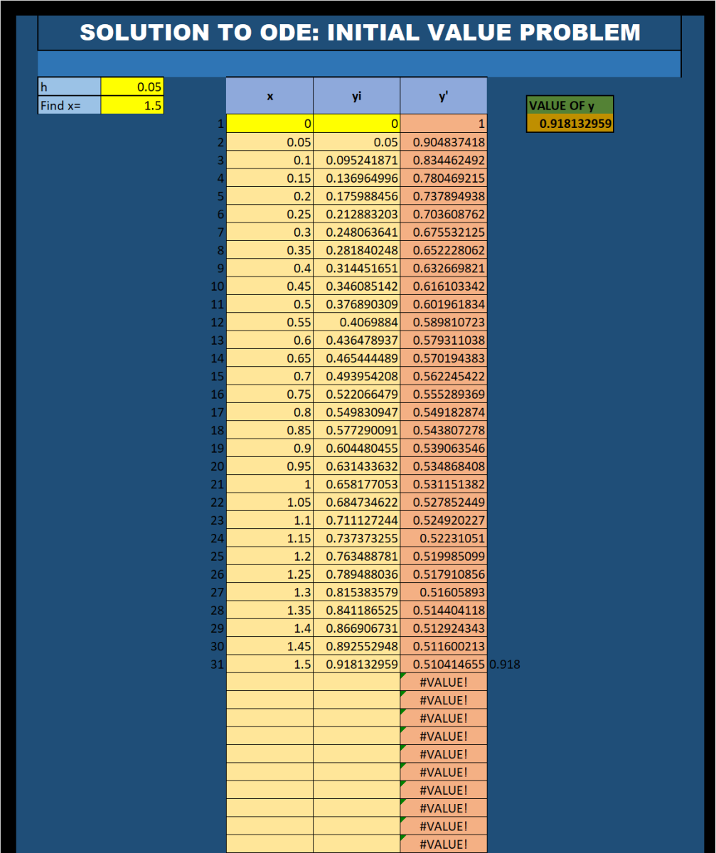
The Algorithm:

1. Start at the known point: (x₀, y₀) = (0, 0)

2. Calculate the current slope:

   y'₀ = e^(-4(0) + 2(0)) = e^0 = 1
   

3. Take a small step forward:

   x₁ = x₀ + h = 0 + 0.05 = 0.05
   y₁ = y₀ + h × y'₀ = 0 + 0.05 × 1 = 0.05
   

4. Recalculate the slope at the new point:

   y'₁ = e^(-4(0.05) + 2(0.05)) = e^(-0.1) ≈ 0.9048
   

5. Take another step:

   x₂ = 0.05 + 0.05 = 0.10
   y₂ = 0.05 + 0.05 × 0.9048 ≈ 0.0952
   

6. Repeat 24 times until reaching x = 1.2

The Geometric Interpretation

Imagine you're hiking in dense fog where you can only see a few meters ahead:

• Your compass (y') tells you which direction to walk at your current position
• Your step size (h) is how far you walk before checking your compass again
• Each step you walk in a straight line in the direction your compass indicates
• The path you trace approximates the true solution curve

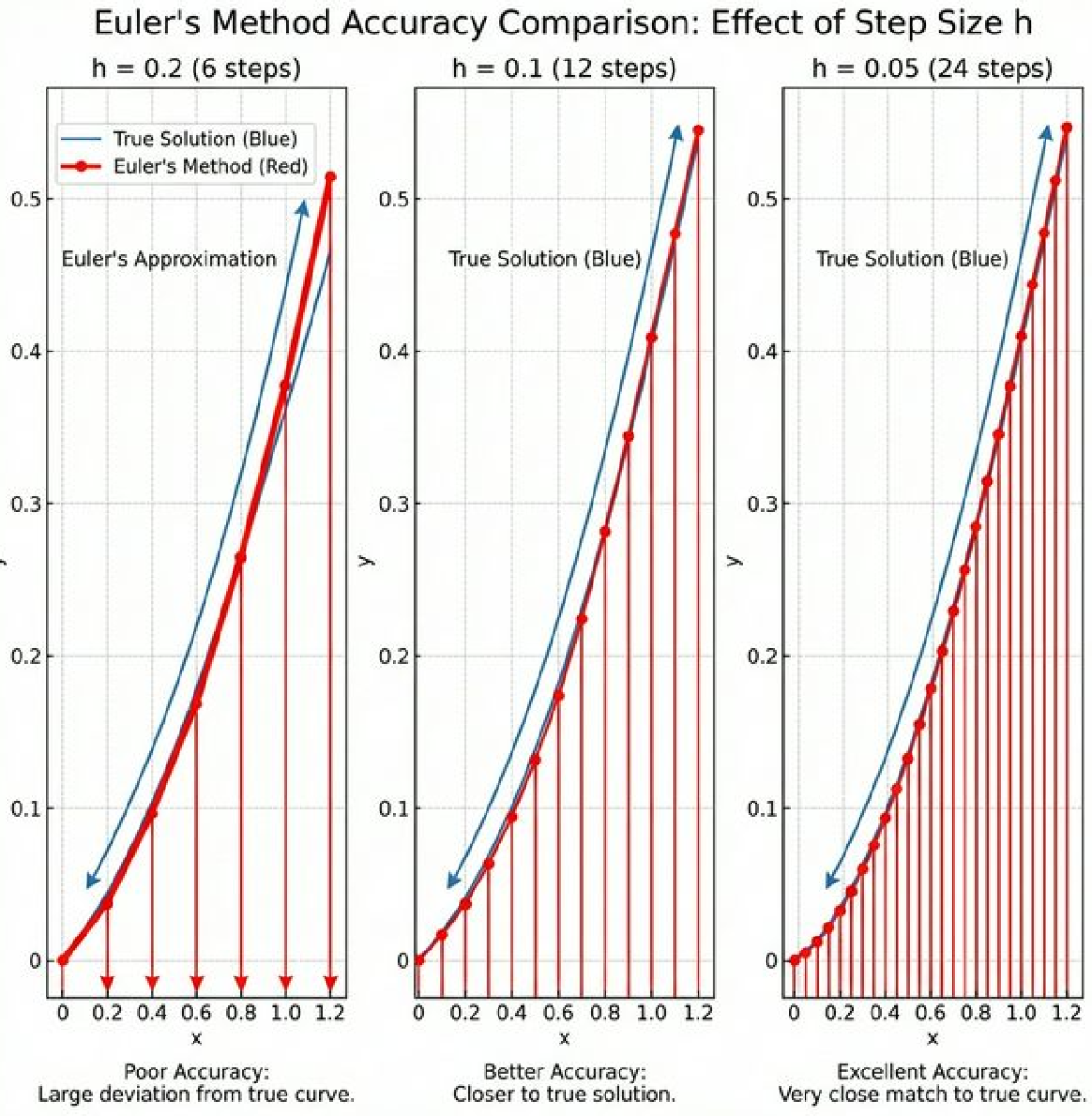
The true solution is a smooth curve, but Euler's Method approximates it with many small straight-line segments. The smaller the steps (smaller h), the closer your approximation follows the true curve.

What This Calculation Can Be Used For

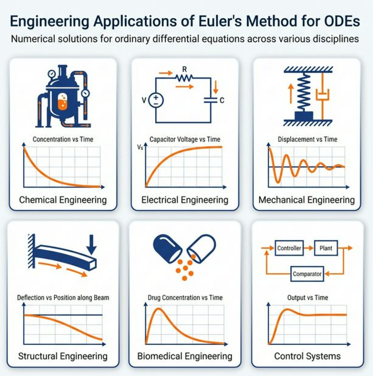
1. Chemical Engineering Applications

Reaction Kinetics:

• Problem: Predicting concentration of reactants over time in non-linear reactions
• Example: In a reactor, if the reaction rate depends exponentially on temperature and concentration
• Use: Design reactor size, predict completion time, optimize operating conditions

Batch Process Design:

• Track how chemical concentrations evolve during batch processing
• Determine when to terminate reactions for optimal yield

2. Electrical Engineering Applications

Non-Linear Circuit Analysis:

• Problem: Current/voltage in circuits with diodes, transistors, or other non-linear components
• Example: Charging/discharging capacitors through semiconductor devices
• Use: Predict circuit behavior, design timing circuits, analyze power supplies

Signal Processing:

• Model non-linear filters and signal transformations
• Predict transient responses in complex electronic systems

3. Mechanical Engineering Applications

Vibration and Damping:

• Problem: Systems with non-linear damping (like shock absorbers)
• Example: Car suspension where damping force depends exponentially on velocity
• Use: Predict oscillation decay, design suspension systems, analyze earthquake response

Heat Transfer:

• Problem: Cooling/heating with radiation (Stefan-Boltzmann law)
• Example: A hot component cooling in air where radiation dominates
• Use: Predict cooling times, design thermal management systems

4. Structural Engineering Applications

Large Deflection Analysis:

• When structural elements undergo deformations where geometry changes significantly
• Cable structures, membrane structures, thin shells

Material Non-Linearity:

• Plastic deformation beyond yield point
• Concrete cracking and progressive failure
• Composite material behavior

5. Environmental Engineering Applications

Pollutant Dispersion:

• Problem: Concentration of pollutants changing through chemical reactions
• Example: Ozone formation in atmosphere with temperature-dependent reaction rates
• Use: Predict air quality, design ventilation systems

Water Treatment:

• Chemical treatment processes with pH-dependent reaction rates
• Biological oxygen demand (BOD) modeling in wastewater

6. Biomedical Engineering Applications

Pharmacokinetics:

• Problem: Drug concentration in bloodstream over time
• Example: Drug elimination rate depending on liver enzyme saturation
• Use: Determine dosing schedules, predict therapeutic windows

Population Dynamics:

• Bacterial growth in bioreactors
• Tumor growth models with carrying capacity

7. Control Systems Engineering

Non-Linear Control:

• Systems where response depends non-linearly on input
• Adaptive control systems
• Robotics with complex dynamics

System Identification:

• Characterizing real-world system behavior
• Model validation and calibration

Practical Engineering Workflow

When Engineers Use This Method:

1. Problem Identification

   • Encounter a rate-of-change problem that can't be solved analytically
   • Formulate the differential equation from physical laws

2. Method Selection

   • Euler's Method: Quick, simple, good for educational purposes or preliminary analysis
   • For production work: More accurate methods (Runge-Kutta, adaptive step size)

3. Implementation

   • Set up spreadsheet (like this ExcelCalcs template)
   • Choose appropriate step size (balance accuracy vs. computation)
   • Verify results with limiting cases or known solutions

4. Analysis

   • Plot solution curve to visualize behavior
   • Identify critical points (maxima, minima, inflection points)
   • Use results for design decisions

Why Use a Spreadsheet Template?

Advantages:

• Transparent: Every calculation step is visible for verification
• Flexible: Easy to modify equation, initial conditions, or step size
• Educational: Shows exactly how numerical methods work
• No Programming: Accessible to engineers without coding experience
• Immediate Results: See the entire solution path at once

This ExcelCalcs Template Specifically:

• Pre-formatted for Euler's Method
• Clear column organization (x, y, y')
• Easy to modify the differential equation in the y' column
• Automatic propagation through all steps
• Visual verification of convergence

Limitations and Considerations

Accuracy Issues:

• Error accumulates with each step (local truncation error)
• Stability concerns for stiff equations (rapidly changing solutions)
• May need very small step sizes for acceptable accuracy

When to Use More Advanced Methods:

• Runge-Kutta methods (RK4): Much better accuracy for similar computational cost
• Adaptive step size methods: Automatically adjust h for efficiency
• Specialized ODE solvers: For stiff equations, boundary value problems

Engineering Judgment:

• Always verify results make physical sense
• Check limiting cases (what happens as x→0 or x→∞?)
• Compare with experimental data when available
• Consider whether numerical error is acceptable for your design margins

Summary

This calculation template provides engineers with a practical, transparent tool for solving differential equations that arise throughout engineering practice. While Euler's Method is the simplest numerical approach, this template demonstrates the fundamental principle behind all numerical ODE solvers: break a complex continuous problem into many simple discrete steps.

For preliminary design, education, and quick analysis, this spreadsheet approach is ideal. For critical production calculations, engineers would typically use more sophisticated methods, but the underlying principle remains the same as demonstrated here.