
Strain-Life Fatigue Parameters from Tensile Properties (for ANSYS)
 (0/0)

Description
Strain–Life Fatigue Parameters from Tensile Properties (for ANSYS)
This workbook estimates the strain–life (Coffin–Manson–Basquin) fatigue coefficients of a metal from its static tensile properties, as needed for a strain–life fatigue analysis in ANSYS or a similar program. It then finds the fatigue life for a given strain or stress amplitude, or the strain and stress amplitudes for a given life, with a correction for mean stress.
Method
The fatigue strength coefficient σ′f, strength exponent b, ductility coefficient ε′f and ductility exponent c are estimated by one of three correlations: Manson's universal slopes, the modified universal slopes of Muralidharan and Manson, or Manson's four-point correlation, using the true fracture ductility D = −ln(1 − ψ). The cyclic stress–strain constants follow from compatibility: n′ = b/c and K′ = σ′f / ε′fn′. Life is related to strain amplitude by
εa = ((σ′f − σm)/E)(2Nf)b + ε′f(2Nf)c (Morrow), or the Smith–Watson–Topper parameter σmaxεa.
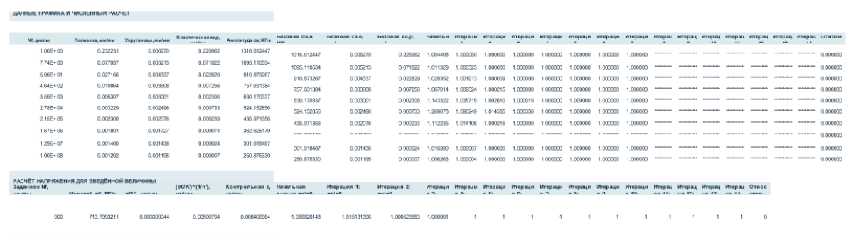
The equations are solved in the cells by Newton iteration and bisection; no Solver or macros are needed.
Inputs
- Young's modulus E and ultimate tensile strength σu (MPa), reduction of area ψ (%)
- Estimation method and mean-stress correction (Morrow or SWT), from drop-down lists
- Stress ratio Rσ
- Solve mode (by cycles, by strain or by stress) and the value given
Outputs
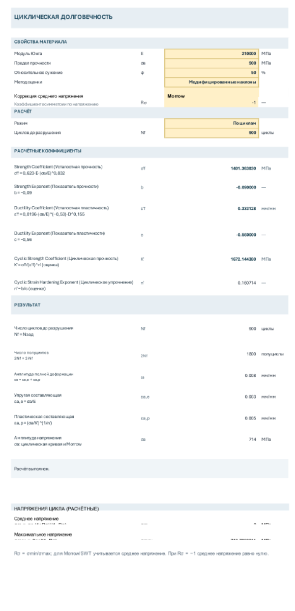
- σ′f, b, ε′f, c, K′ and n′, each with its formula shown
- Cycles to failure Nf, total, elastic and plastic strain amplitudes, stress amplitude, mean and maximum stress
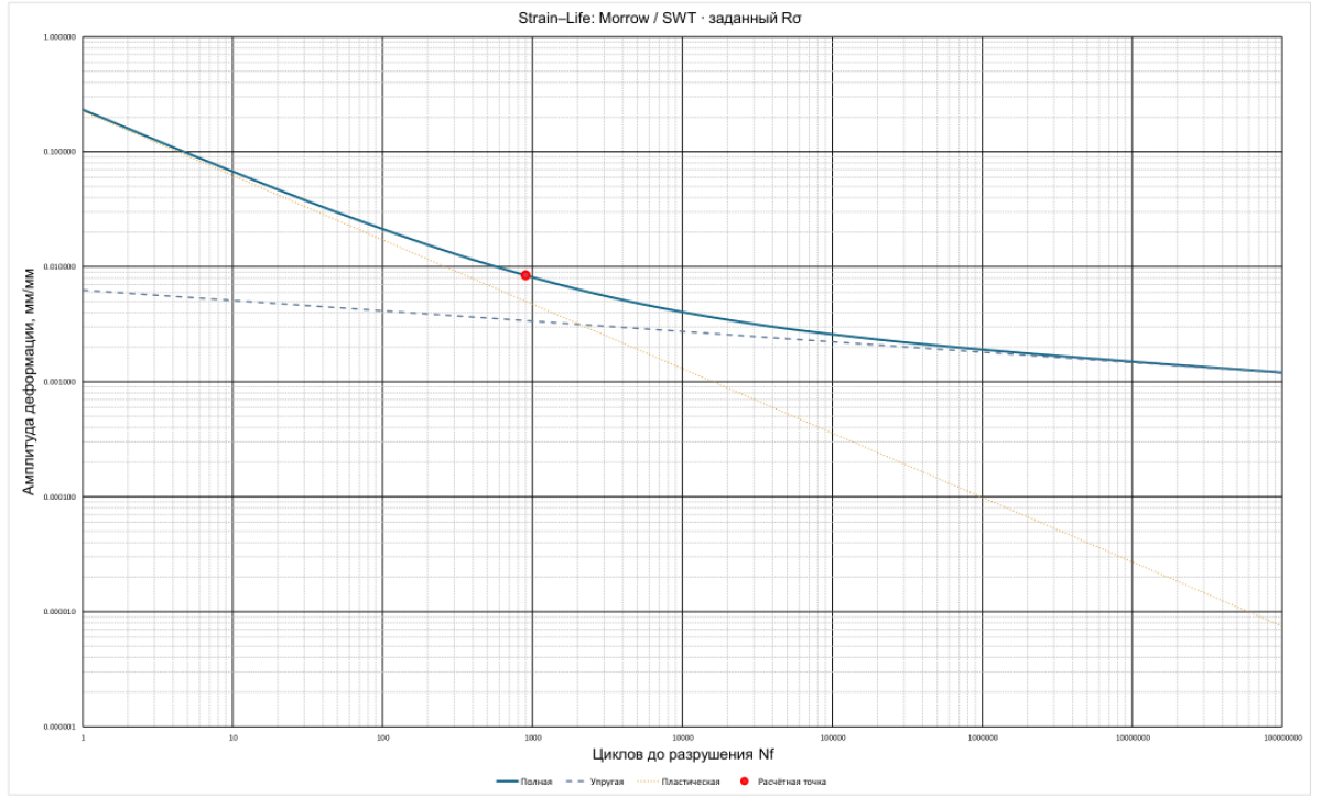
- A strain–life chart with the design point
Checked
For the stored example (E = 210,000 MPa, σu = 900 MPa, ψ = 50%, modified universal slopes, R = −1, Nf = 900) an independent calculation gives the same σ′f = 1,401.4 MPa, ε′f = 0.3331, K′ = 1,672.1 MPa, n′ = 0.1607, stress amplitude 713.8 MPa and strain amplitude 0.008407; solving back from that strain returns Nf = 900.
Please note
- The worksheet is in Russian; the equations are printed in standard notation.
- The coefficients are estimates from static properties. Use measured strain–life data where it is available.
Calculation Preview
 (0/0)
Full download access to any calculation is available to users with a paid or awarded subscription (XLC Pro).
Subscriptions are free to contributors to the site, alternatively they can be purchased.
Click here for information on subscriptions.
I also reviewed the calculation against our Good Calculation Guide: [https://www.excelcalcs.com/calcs/good-calc-guide](https://www.excelcalcs.com/calcs/good-calc-guide)
**What works well**
- Each coefficient is shown with its formula, so the method can be followed at a glance.
- Drop-down lists for the method, the mean-stress correction and the solve mode, and every input is validated with a clear error message.
- The iterations are done in the cells, with a convergence check, so no Solver or macros are needed.
- The strain–life chart responds to the inputs and marks the design point.
**Suggestions that would make it even better**
- Say how it was validated, for example by comparing the coefficients with published values for a well-known steel.
- Cite the source of each correlation (Manson's universal slopes, Muralidharan and Manson's modified slopes, the four-point correlation, Morrow, Smith–Watson–Topper).
- State the purpose at the top, including which ANSYS strain–life fields the results go into.
- Add cell comments explaining each input and the three solve modes.
- Try the XLC add-in, which shows each formula as an equation so readers can check it at a glance.
If you send in an updated version that covers these points, it would qualify for our 12-month XLC Pro award.