Combined
0 ContainersFiles in Combined
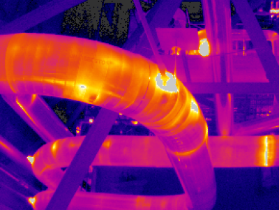
Conduction-Convection and Radiation from Pipes
Calculation Reference Heat Loss from Pipes
Heat Transfer
Fliuid Flow in Pipes
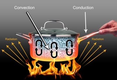
Conduction, convection, and radiatio...
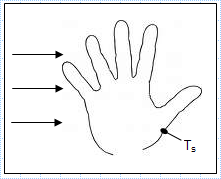
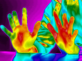
Hand experiencing convection heat transfer with moving air and water.xls
KNOWN: Hand experiencing convection heat transfer with moving air and water.
FIND: Determine which condition feels colder. Contrast th...
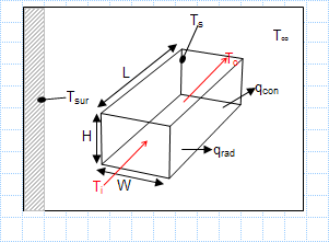
Heat loss in duct.xls
KNOWN: Dimensions, average surface temperature and emissivity of heating duct. Duct air inlet temperature and velocity. Temperature of ambi...
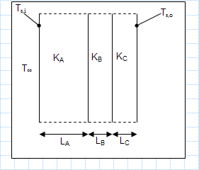
Heat loss through a composite wall of three materials.xls
KNOWN: Thicknesses of three materials which form a composite wall and thermal conductivities of the two materials. Inner and outer surface ...
Heat loss through single pane of glass.xls
KNOWN: Temperature and convection coefficients associated with air at the inner and outer surfaces of a rear window.
FIND: a) Inner an...
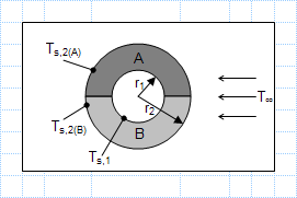
Heat transfer by conduction and convection - electrical circuit analogy.xls
KNOWN: Inner surface temperature of insulation blanket comprised of two semi-cylindrical shells of different materials. Ambient air conditi...
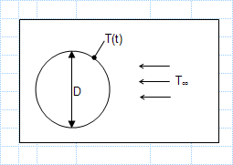
Heat transfer coefficient between sphere and air stream.xls
KNOWN: The Temperature-time history of a pure copper sphere in an air stream.
FIND: The heat transfer coefficient between the sphere a...

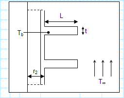
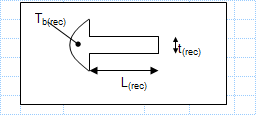
Heat transfer in cooling fins.xls
KNOWN: Dimensions and base temperature of aluminum fins of rectangular profile. Ambient air conditions. FIND: a) Fin efficiency and effect...
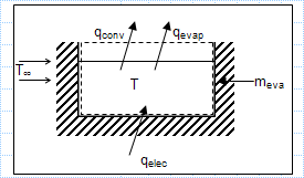
Mass and heat transfer - evaparation.xls
KNOWN: Operating temperature, ambient air conditions and make-up water requirements for a hot tub.
FIND: Heater power required to main...
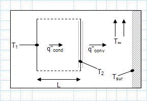
Radiation and convection heat transfer to large surroundings.xls
KNOWN: Thickness and thermal conductivity, k, of an oven wall. Temperature and emissivity,?, of front surface. Temperature and convection ...
Rectangular verses triangular cooling fin effectiveness.xls
KNOWN: Dimensions, base temperature and environmental conditions associated with rectangular and triangular stainless steel fins. FIND: Ef...
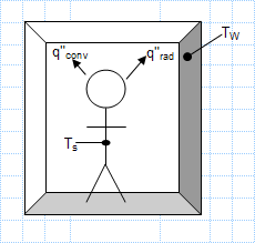
Surface temperature convection coefficient and emissivity of a person in the room.xls
KNOWN: Air and wall temperatures of a room. Surface temperature, convection coefficient and emissivity of a person in the room.
FIND: ...

ThermalTransient1D.xls
